Inferring the progenitor of a recoiling SMBH: JWST RBH-1

RBH-1 is a candidate recoiling supermassive black hole identified in HST/JWST imaging by Islam, Venumadhav & Wadekar (2026, arXiv:2601.18986), with an inferred recoil velocity of

\[v_{\rm kick} = 954^{+110}_{-126}\ {\rm km\,s^{-1}}.\]

Such a large recoil can only come from a fairly specific progenitor — high, misaligned spins and near-comparable masses. We infer the progenitor mass ratio and spin magnitudes from the measured kick with gwGenealogy.core.KickToProgenitor, which inverts the IW2025 precessing-kick flow.

The flow is a conditional density \(p(v_{\rm kick}\,|\,q, a_1, a_2)\) (spin angles marginalised internally). KickToProgenitor uses it as a likelihood and applies Bayes,

\[p(q,a_1,a_2\,|\,d) \propto \Big[\int p(d\,|\,v)\,p(v\,|\,q,a_1,a_2)\,dv\Big]\,\pi(q,a_1,a_2),\]

marginalising the (asymmetric) measurement uncertainty \(p(d\,|\,v)\) and importance-sampling over the prior \(\pi\).

import warnings
warnings.filterwarnings('ignore', 'Wswiglal-redir-stdio')

import numpy as np
import matplotlib.pyplot as plt

from gwGenealogy.core import KickToProgenitor
from gwGenealogy.utils import set_rcparams

set_rcparams()

lal.MSUN_SI != Msun

Set up and run the inversion

The \(954^{+110}_{-126}\) km/s error bar is asymmetric, so we pass sigma_lo=126 and sigma_hi=110 — KickToProgenitor models the measurement as a split normal and marginalises over the true kick. Priors: \(q\sim\mathcal{U}[1,20]\), \(a_1, a_2\sim\mathcal{U}[0,1]\) (the defaults).

k2p = KickToProgenitor(
    v_kicks=954.0, sigma_lo=126.0, sigma_hi=110.0,
    q_min=1.0, q_max=20.0,            # spins default to U[0, 1]
    n_prior=300_000, n_posterior=40_000, seed=0)
print(k2p)

results = k2p.infer(verbose=True)

summary = k2p.summary(ci=90)
print('\nRBH-1 progenitor (median, 90% CI):')
for p in ('q', 'a1', 'a2'):
    print(f'  {p:>3s} = {summary[p + "_median"][0]:5.2f}  '
          f'[{summary[p + "_low"][0]:.2f}, {summary[p + "_high"][0]:.2f}]')

KickToProgenitor(n_kicks=1, Gaussian errors, n_prior=300000, n_posterior=40000)
  kick 1/1: v=954 km/s  ESS=40805/300000  -> q=3.01, a1=0.79, a2=0.52

RBH-1 progenitor (median, 90% CI):
    q =  3.01  [1.17, 6.88]
   a1 =  0.79  [0.41, 0.98]
   a2 =  0.52  [0.05, 0.93]

Progenitor posterior

fig, axes = k2p.plot_posteriors(index=0)
plt.show()

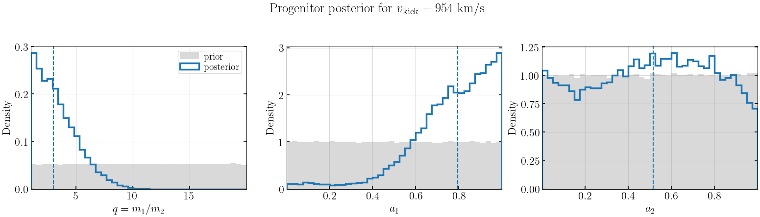
The large recoil drives the primary spin high (\(a_1 \approx 0.8\), disfavouring \(a_1 \lesssim 0.4\)) and favours comparable masses (\(q\) peaks near 2–3). The secondary spin \(a_2\) is only weakly constrained. The \(q\) posterior sits well below the prior’s upper edge, so the \(q \le 20\) bound is immaterial and we stay within the flow’s calibrated range (\(q \lesssim 14\)).

Posterior-predictive check

posterior_predictive draws one kick from each posterior progenitor. Because the flow marginalises over spin orientation, a single \((q, a_1, a_2)\) maps to a broad kick distribution — the same progenitor can recoil at very different speeds depending on the (unobserved) spin geometry. So the predictive distribution is wide and not sharply peaked at 954 km/s: the inference constrains masses and spin magnitudes, not the spin angles that set the exact recoil.

vk_pp = k2p.posterior_predictive(index=0, n=20000, seed=1)

fig, ax = plt.subplots(figsize=(7, 4.5))
ax.hist(vk_pp, bins=80, density=True, alpha=0.6, label='posterior-predictive')
ax.axvline(954, color='C3', ls='--', lw=2, label=r'observed $954$ km/s')
ax.axvspan(954 - 126, 954 + 110, color='C3', alpha=0.15)
ax.set_xlabel(r'$v_{\rm kick}$ [km/s]'); ax.set_ylabel('Density')
ax.set_title('Posterior-predictive kicks vs the RBH-1 measurement')
ax.legend(frameon=False)
plt.tight_layout(); plt.show()

print(f'posterior-predictive kick: median={np.median(vk_pp):.0f}  '
      f'90% CI=[{np.percentile(vk_pp, 5):.0f}, {np.percentile(vk_pp, 95):.0f}] km/s')

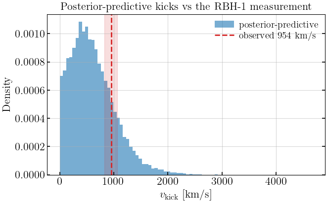
posterior-predictive kick: median=554  90% CI=[72, 1375] km/s

Many kicks at once

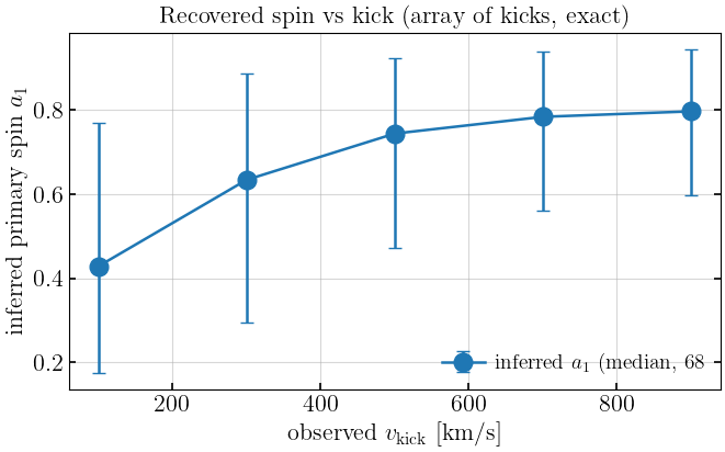
KickToProgenitor accepts an array of kicks and returns a posterior for each (here treated as exact, sigma=None). The inferred primary spin rises monotonically with the recoil — the expected trend.

v_arr = np.array([100, 300, 500, 700, 900])
multi = KickToProgenitor(v_arr, q_min=1, q_max=20,
                         n_prior=200_000, n_posterior=20_000, seed=0)
multi.infer()
ms = multi.summary(ci=68)

fig, ax = plt.subplots(figsize=(7, 4.5))
ax.errorbar(v_arr, ms['a1_median'],
            yerr=[ms['a1_median'] - ms['a1_low'], ms['a1_high'] - ms['a1_median']],
            fmt='C0-o', capsize=4, label=r'inferred $a_1$ (median, 68%)')
ax.set_xlabel(r'observed $v_{\rm kick}$ [km/s]')
ax.set_ylabel(r'inferred primary spin $a_1$')
ax.set_title('Recovered spin vs kick (array of kicks, exact)')
ax.legend(frameon=False)
plt.tight_layout(); plt.show()

Caveats

• Posterior, not a unique progenitor. The recoil is a many-to-one function of \((q, a_1, a_2)\) and the spin angles, so the widths above are real physical degeneracy.

• Spin tilts are unrecoverable. The flow’s context is only \((q, a_1, a_2)\); the tilt/azimuth dependence is marginalised inside it. We constrain spin magnitudes and mass ratio, never the orientations.

• Prior-dependent. KickToProgenitor takes a range + distribution or an explicit prior array per parameter; an astrophysically motivated SMBH-merger prior would sharpen or shift the result. Watch the ess — kicks in the model’s far tail thin the prior pool and need a larger n_prior.

• Single-event inference. Each kick is treated independently; a population of recoiling SMBHs would call for hierarchical inference.