BHPTNRSur1dq1e4-gwNRHME model#
BHPTNRSur1dq1e4-gwNRHME is a non-spinning eccentric binary black hole merger mulit-modal waveform model. We obtain BHPTNRSur1dq1e4-gwNRHME predictions by combining quadrupolar eccentric model EccentricIMR and circular waveform model BHPTNRSur1dq1e4 using gwNRHME framework.
BHPTNRSur1dq1e4-gwNRHME (multi-modal eccentric nonspinning model) = EccentricIMR (22 mode eccentric nonspinning model) + BHPTNRSur1dq1e4 (multi-modal circular nonspinning model) + gwNRHME framework
import warnings
warnings.filterwarnings("ignore", "Wswiglal-redir-stdio")
import matplotlib.pyplot as plt
import numpy as np
import gwtools

# import gwModels
import sys
PATH_TO_GWMODELS = "/home/tousifislam/Documents/works/git_repos/gwModels/"
sys.path.append(PATH_TO_GWMODELS)
import gwModels
lal.MSUN_SI != Msun
__name__ = gwsurrogate.new.spline_evaluation
__package__= gwsurrogate.new
Loaded NRHybSur3dq8 model
Setup your mathematica kernel#
To setup the Mathematica kkernel, we need to know the path to your Wolfram kernel and path to the directory containing the EccentricIMR package.
# Set the path to your Wolfram kernel
wolfram_kernel_path = '/home/tousifislam/Documents/Mathematica/ScriptDir/WolframKernel'

# Set the path to the directory containing the EccentricIMR package
package_directory = PATH_TO_GWMODELS + '/externals/EccentricIMR2017/'
Setup your gwsurrogate module for BHPTNRSur#
import gwsurrogate
# setup model for BHPTNRSur1dq1e4
path_to_gws = '/home/tousifislam/miniconda3/envs/eccentric/lib/python3.9/site-packages/gwsurrogate/'
path_to_surrogate = path_to_gws+'surrogate_downloads/BHPTNRSur1dq1e4.h5'
model = gwsurrogate.EvaluateSurrogate(path_to_surrogate, ell_m=[(2,2),(2,1),(3,1),(3,2),(3,3),(4,2),(4,3),(4,4),(5,3),(5,4),(5,5)])
loading surrogate mode... l2_m2

>>> Found surrogate ID from file name: BHPTNRSur1dq1e4

>>> Warning: Guessing quadrature weights to be identical with 0.200000
Cannot load greedy points...OK
Special case: using spline for parametric model at each EI node
num_fits_amp = 7
num_fits_phase = 7
setting norm fitparams to None...
loading surrogate mode... l2_m1

>>> Found surrogate ID from file name: BHPTNRSur1dq1e4

>>> Warning: Guessing quadrature weights to be identical with 0.200000
Cannot load greedy points...OK
Special case: using spline for parametric model at each EI node
num_fits_re = 13
num_fits_im = 13
setting norm fitparams to None...
loading surrogate mode... l3_m1

>>> Found surrogate ID from file name: BHPTNRSur1dq1e4

>>> Warning: Guessing quadrature weights to be identical with 0.200000
Cannot load greedy points...OK
Special case: using spline for parametric model at each EI node
num_fits_re = 13
num_fits_im = 13
setting norm fitparams to None...
loading surrogate mode... l3_m2

>>> Found surrogate ID from file name: BHPTNRSur1dq1e4

>>> Warning: Guessing quadrature weights to be identical with 0.200000
Cannot load greedy points...OK
Special case: using spline for parametric model at each EI node
num_fits_re = 13
num_fits_im = 13
setting norm fitparams to None...
loading surrogate mode... l3_m3

>>> Found surrogate ID from file name: BHPTNRSur1dq1e4

>>> Warning: Guessing quadrature weights to be identical with 0.200000
Cannot load greedy points...OK
Special case: using spline for parametric model at each EI node
num_fits_re = 13
num_fits_im = 13
setting norm fitparams to None...
loading surrogate mode... l4_m2

>>> Found surrogate ID from file name: BHPTNRSur1dq1e4

>>> Warning: Guessing quadrature weights to be identical with 0.200000
Cannot load greedy points...OK
Special case: using spline for parametric model at each EI node
num_fits_re = 13
num_fits_im = 13
setting norm fitparams to None...
loading surrogate mode... l4_m3

>>> Found surrogate ID from file name: BHPTNRSur1dq1e4

>>> Warning: Guessing quadrature weights to be identical with 0.200000
Cannot load greedy points...OK
Special case: using spline for parametric model at each EI node
num_fits_re = 13
num_fits_im = 13
setting norm fitparams to None...
loading surrogate mode... l4_m4

>>> Found surrogate ID from file name: BHPTNRSur1dq1e4

>>> Warning: Guessing quadrature weights to be identical with 0.200000
Cannot load greedy points...OK
Special case: using spline for parametric model at each EI node
num_fits_re = 13
num_fits_im = 13
setting norm fitparams to None...
loading surrogate mode... l5_m3

>>> Found surrogate ID from file name: BHPTNRSur1dq1e4

>>> Warning: Guessing quadrature weights to be identical with 0.200000
Cannot load greedy points...OK
Special case: using spline for parametric model at each EI node
num_fits_re = 13
num_fits_im = 13
setting norm fitparams to None...
loading surrogate mode... l5_m4

>>> Found surrogate ID from file name: BHPTNRSur1dq1e4

>>> Warning: Guessing quadrature weights to be identical with 0.200000
Cannot load greedy points...OK
Special case: using spline for parametric model at each EI node
num_fits_re = 13
num_fits_im = 13
setting norm fitparams to None...
loading surrogate mode... l5_m5

>>> Found surrogate ID from file name: BHPTNRSur1dq1e4

>>> Warning: Guessing quadrature weights to be identical with 0.200000
Cannot load greedy points...OK
Special case: using spline for parametric model at each EI node
num_fits_re = 13
num_fits_im = 13
setting norm fitparams to None...
Surrogate interval [[0.39794001]
 [4.        ]]
Surrogate time grid [-30500.         -30499.8        -30499.6        ...    114.40000011
    114.60000011    114.80000011]
Surrogate parameterization map from q to log10(q)

  Surrogates with this parameterization expect its user intput
  to be the mass ratio q.

  The surrogate will map q to the internal surrogate's
  parameterization which is log10(q)

  The surrogates training interval is quoted in log10(q).
Generate waveforms from combined eccentric models#
# Set the binary parameters
params = {"q": 2.6, # mass ratio
          "x0": 0.07, # reference initial dimensionless orbital frequency
          "e0": 0.1, # initial eccentricity
          "l0": 0, # initial mean anomaly
          "phi0": 0, # initial reference phase
          "t0": 0} # some initial reference time - not much relevant for us
# instantiate the EccentricIMR HM class - it may take some time
# it generate waveforms by combining EccentricIMR and BHPTNRSur1dq1e4
wf = gwModels.BHPTNRSur1dq1e4_gwNRHME(wolfram_kernel_path, package_directory, model=model)

# waveform
tNRE, hNRE = wf.generate_waveform(params)
Times[1.0, 0] is too small to represent as a normalized machine number; precision may be lost.
Times[1.0, 0] is too small to represent as a normalized machine number; precision may be lost.
Times[1.0, 0] is too small to represent as a normalized machine number; precision may be lost.
Further output of MessageName[General, munfl] will be suppressed during this calculation.
Times[1.0, 0] is too small to represent as a normalized machine number; precision may be lost.
Times[1.0, 0] is too small to represent as a normalized machine number; precision may be lost.
Times[1.0, 0] is too small to represent as a normalized machine number; precision may be lost.
Times[1.0, 0] is too small to represent as a normalized machine number; precision may be lost.
Further output of MessageName[General, munfl] will be suppressed during this calculation.
Times[1.0, 0] is too small to represent as a normalized machine number; precision may be lost.
# print available modes
print(hNRE.keys())
dict_keys(['h_l2m2', 'h_l2m1', 'h_l3m3', 'h_l3m2', 'h_l4m4', 'h_l4m3'])
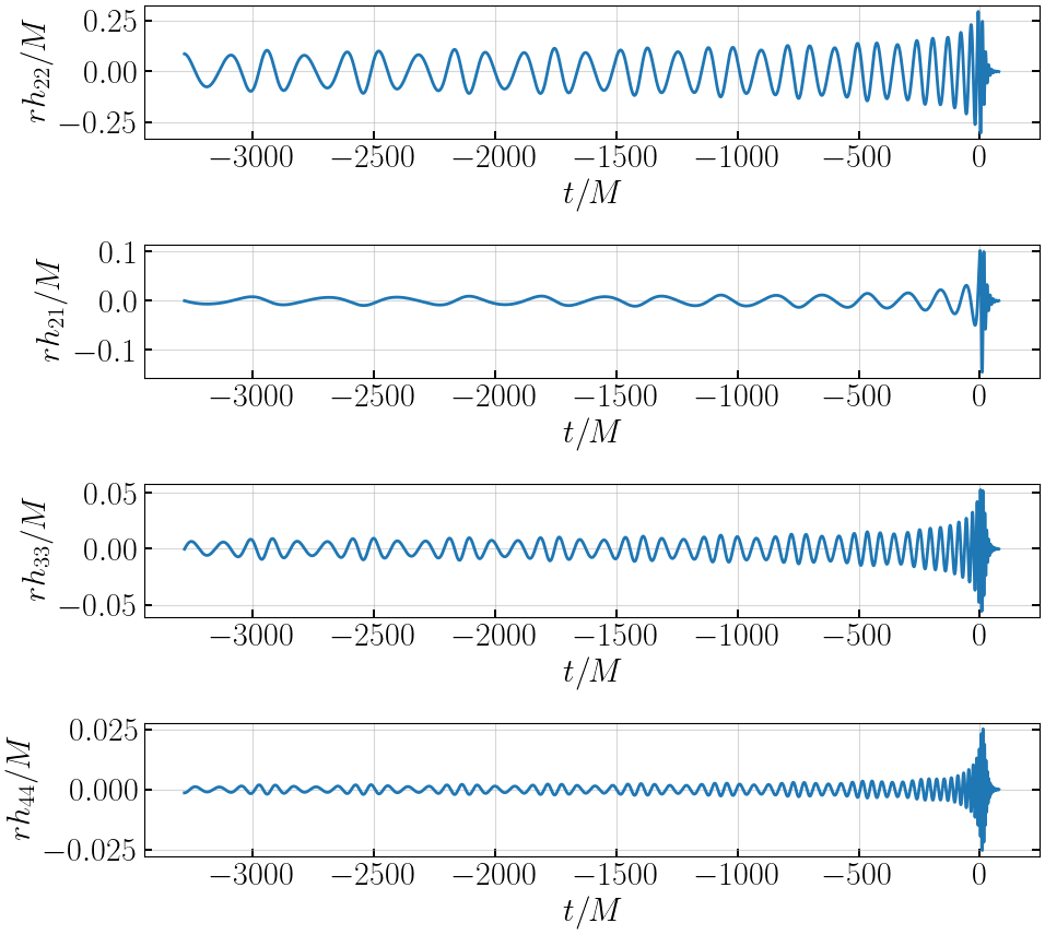
# plot waveform
plt.figure(figsize=(10,9))
plt.subplot(411)
plt.plot(tNRE, hNRE['h_l2m2'], '-', lw=2, label='EccentricIMR')
plt.xlabel('$t/M$')
plt.ylabel('$rh_{22}/M$')
plt.subplot(412)
plt.plot(tNRE, hNRE['h_l2m1'], '-', lw=2, label='EccentricIMR')
plt.xlabel('$t/M$')
plt.ylabel('$rh_{21}/M$')
plt.subplot(413)
plt.plot(tNRE, hNRE['h_l3m3'], '-', lw=2, label='EccentricIMR')
plt.xlabel('$t/M$')
plt.ylabel('$rh_{33}/M$')
plt.subplot(414)
plt.plot(tNRE, hNRE['h_l4m4'], '-', lw=2, label='EccentricIMR')
plt.xlabel('$t/M$')
plt.ylabel('$rh_{44}/M$')
plt.tight_layout()
plt.show()
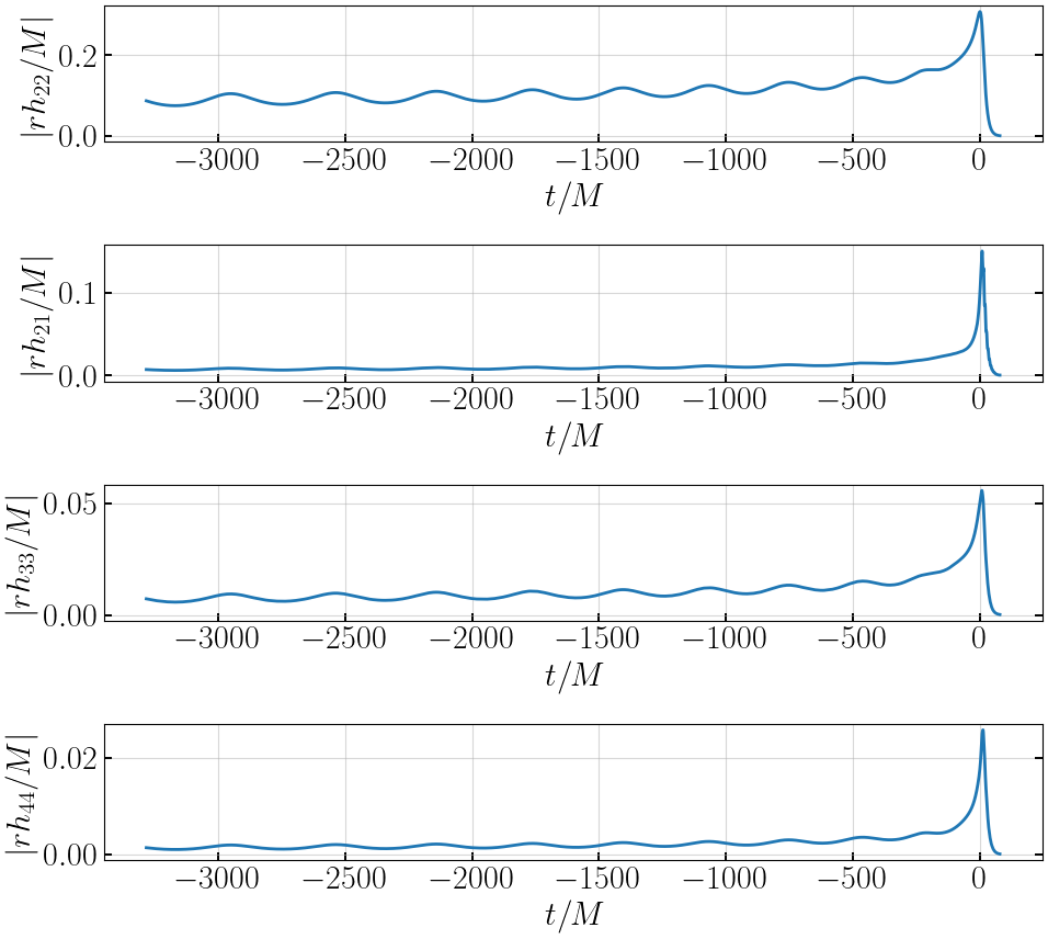
# plot amplitudes
plt.figure(figsize=(10,9))
plt.subplot(411)
plt.plot(tNRE, abs(hNRE['h_l2m2']), '-', lw=2, label='EccentricIMR')
plt.xlabel('$t/M$')
plt.ylabel('$|rh_{22}/M|$')
plt.subplot(412)
plt.plot(tNRE, abs(hNRE['h_l2m1']), '-', lw=2, label='EccentricIMR')
plt.xlabel('$t/M$')
plt.ylabel('$|rh_{21}/M|$')
plt.subplot(413)
plt.plot(tNRE, abs(hNRE['h_l3m3']), '-', lw=2, label='EccentricIMR')
plt.xlabel('$t/M$')
plt.ylabel('$|rh_{33}/M|$')
plt.subplot(414)
plt.plot(tNRE, abs(hNRE['h_l4m4']), '-', lw=2, label='EccentricIMR')
plt.xlabel('$t/M$')
plt.ylabel('$|rh_{44}/M|$')
plt.tight_layout()
plt.show()
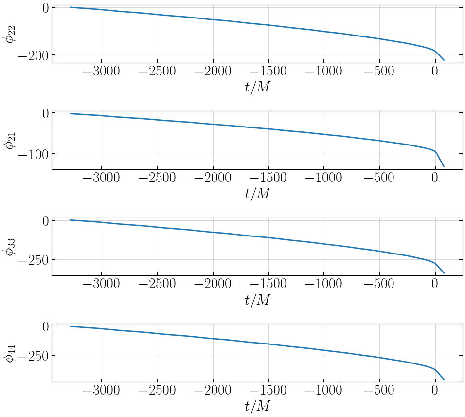
# plot phases
plt.figure(figsize=(10,9))
plt.subplot(411)
plt.plot(tNRE, gwtools.phase(hNRE['h_l2m2']), '-', lw=2, label='EccentricIMR')
plt.xlabel('$t/M$')
plt.ylabel('$\\phi_{22}$')
plt.subplot(412)
plt.plot(tNRE, gwtools.phase(hNRE['h_l2m1']), '-', lw=2, label='EccentricIMR')
plt.xlabel('$t/M$')
plt.ylabel('$\\phi_{21}$')
plt.subplot(413)
plt.plot(tNRE, gwtools.phase(hNRE['h_l3m3']), '-', lw=2, label='EccentricIMR')
plt.xlabel('$t/M$')
plt.ylabel('$\\phi_{33}$')
plt.subplot(414)
plt.plot(tNRE, gwtools.phase(hNRE['h_l4m4']), '-', lw=2, label='EccentricIMR')
plt.xlabel('$t/M$')
plt.ylabel('$\\phi_{44}$')
plt.tight_layout()
plt.show()