Example notebook to use gwNRHME framework

This framework is developed in https://arxiv.org/abs/2403.15506.

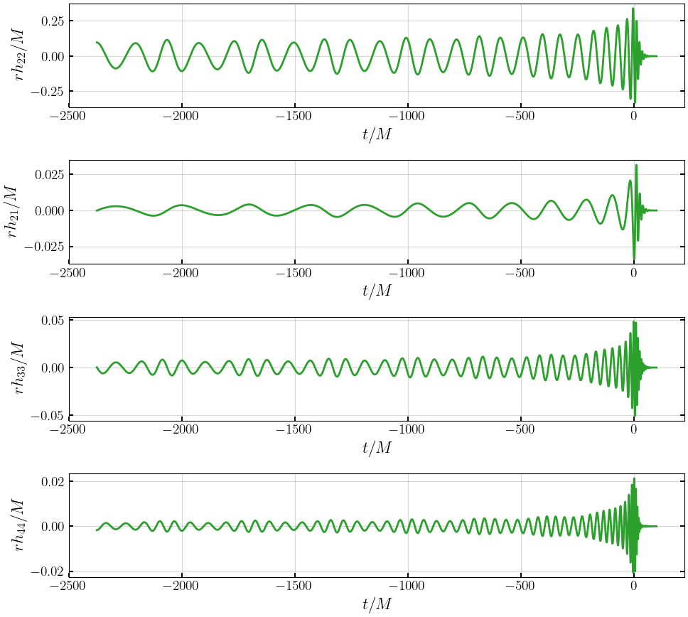
Utilizing publicly available non-spinning eccentric binary black hole (BBH) merger simulations from the SXS collaboration, we presents convincing evidence that the waveform phenomenology in eccentric BBH mergers is significantly simpler than previously thought. We find that the eccentric modulations in the amplitudes, phases, and frequencies in different spherical harmonic modes are all related and can be modeled using a single time series modulation. Using this universal eccentric modulation, we provide a framework named gwNRHME to seamlessly convert a multi-modal (i.e with several spherical harmonic modes) quasi-circular waveform into multi-modal eccentric waveform if the quadrupolar eccentric waveform is known. This reduces the modelling complexity of eccentric BBH mergers drastically as we now have to model only a single eccentric modulation time-series instead of modelling the effect of eccentricity in all modes. When compared with the NR simulations, our framework mismatches are mostly ~0.001 and are comparable to the numerical errors in the NR simulations. Our method is modular and can be readily added to any quadrupolar non-spinning eccentric waveform model.

import sys
# install gwModels in editable mode from the parent directory
!{sys.executable} -m pip install -e ../ --no-deps --quiet

import matplotlib.pyplot as plt
import numpy as np
import warnings
warnings.filterwarnings("ignore", "Wswiglal-redir-stdio")

import gwModels
gwModels.utils.set_rcparams()

lal.MSUN_SI != Msun

1. Generate eccentric 22 mode waveform

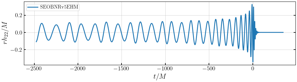
We use the SEOBNRv5EHM model via pyseobnr to generate the eccentric quadrupolar waveform.

# instantiate the SEOBNRv5EHM class
seob = gwModels.waveforms.genSEOBNRv5EHM()

# Set the binary parameters
params = {"q": 2,       # mass ratio
          "omega0": 0.02, # initial dimensionless orbital frequency
          "e0": 0.1,     # initial eccentricity
          "l0": 0}       # initial relativistic anomaly

# generate eccentric waveform modes
tecc, hecc_dict = seob.generate_SEOBNRv5EHM(params)
hecc = hecc_dict['h_l2m2']

# plot waveform
plt.figure(figsize=(10,3))
plt.plot(tecc, hecc.real, '-', lw=2, color='C0', label='SEOBNRv5EHM')
plt.xlabel('$t/M$')
plt.ylabel('$rh_{22}/M$')
plt.legend()
plt.tight_layout()
plt.show()

2. Generate multi-modal circular waveform

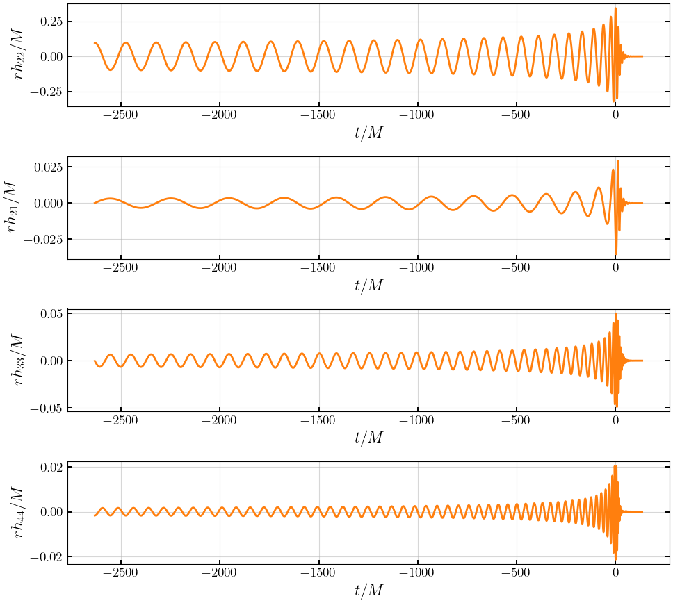
We use NRHybSur3dq to generate circular waveform in the non-spinning limit.

gwsur = gwModels.waveforms.genNRHybSur3dq8()

Loaded NRHybSur3dq8 model

tsur, hsur = gwsur.generate_NRHybSur3dq8(params)
print(hsur.keys())

dict_keys(['h_l2m1', 'h_l2m2', 'h_l3m2', 'h_l4m4', 'h_l3m3', 'h_l3m1', 'h_l4m3', 'h_l4m2', 'h_l5m5'])

# plot waveform
plt.figure(figsize=(10,9))
plt.subplot(411)
plt.plot(tsur, hsur['h_l2m2'].real, '-', lw=2, color='C1', label='NRHybSur3dq8')
plt.xlabel('$t/M$')
plt.ylabel('$rh_{22}/M$')
plt.subplot(412)
plt.plot(tsur, hsur['h_l2m1'].real, '-', lw=2, color='C1', label='NRHybSur3dq8')
plt.xlabel('$t/M$')
plt.ylabel('$rh_{21}/M$')
plt.subplot(413)
plt.plot(tsur, hsur['h_l3m3'].real, '-', lw=2, color='C1', label='NRHybSur3dq8')
plt.xlabel('$t/M$')
plt.ylabel('$rh_{33}/M$')
plt.subplot(414)
plt.plot(tsur, hsur['h_l4m4'].real, '-', lw=2, color='C1', label='NRHybSur3dq8')
plt.xlabel('$t/M$')
plt.ylabel('$rh_{44}/M$')
plt.tight_layout()
plt.show()

3. Combine them to obtain multi-modal eccentric waveforms

gwnrhme = gwModels.frameworks.NRHME(t_ecc = tecc,
                         h_ecc_dict = {'h_l2m2': hecc},
                         t_cir = tsur,
                         h_cir_dict = hsur)

tNRE = gwnrhme.t_common
hNRE = gwnrhme.hNRE

print(hNRE.keys())

dict_keys(['h_l2m2', 'h_l2m1', 'h_l3m2', 'h_l4m4', 'h_l3m3', 'h_l3m1', 'h_l4m3', 'h_l4m2', 'h_l5m5'])

# plot waveform
plt.figure(figsize=(10,9))
plt.subplot(411)
plt.plot(tNRE, hNRE['h_l2m2'].real, '-', lw=2, color='C2', label='gwNRHME')
plt.xlabel('$t/M$')
plt.ylabel('$rh_{22}/M$')
plt.subplot(412)
plt.plot(tNRE, hNRE['h_l2m1'].real, '-', lw=2, color='C2', label='gwNRHME')
plt.xlabel('$t/M$')
plt.ylabel('$rh_{21}/M$')
plt.subplot(413)
plt.plot(tNRE, hNRE['h_l3m3'].real, '-', lw=2, color='C2', label='gwNRHME')
plt.xlabel('$t/M$')
plt.ylabel('$rh_{33}/M$')
plt.subplot(414)
plt.plot(tNRE, hNRE['h_l4m4'].real, '-', lw=2, color='C2', label='gwNRHME')
plt.xlabel('$t/M$')
plt.ylabel('$rh_{44}/M$')
plt.tight_layout()
plt.show()